Differential Privacy as Hypothesis Testing
Published:
Connecting the dots between Differential Privacy, Hypothesis Testing and (ideal) adversaries.
1. Differential Privacy as Hypothesis Testing
Differential Privacy (DP) is the golden standard used both in academia and industry to reason about how private an algorithm is, but its adoption rate is rather small due to unclear guarantees it provides you. Even more, if you decide to use relaxations of DP, like Approximate DP, Renyi-DP, f-DP and so on, you might feel intimidated and a bit lost. In this blog post, I would try to shed some light on what DP is trying to achieve from the lens of an adversary that tries to break our privacy and how DP guarantees to ruin the chances of the attacker to succeed.
Pure Differential Privacy:
Differential privacy claims that an algorithm M provides $\epsilon$-DP privacy if for two databases (collections of data) that differ in one element $D_1$ and $D_2$ and an output space O, the following property holds:
\[P[M(D_1) \in O] < e^\epsilon * P[M(D_2) \in O]\]A nice way of understanding DP is that if algorithm A does not release any kind of information about the existence of a given sample in the database, then the privacy of that sample is protected. A quote that describes best DP is made directly by Dwork and Roth in their seminal book:
Differential privacy describes a promise, made by a data holder, or curator, to a data subject: “You will not be affected, adversely or otherwise, by allowing your data to be used in any study or analysis, no matter what other studies, data sets, or information sources, are available.”

This sounds neat! Before talking about algorithms that try to achieve $\epsilon$-DP and keep their promise to the data subject, let’s discuss about adversaries. To develop a strong defence, we need to understand whom we are protecting against, right (or maybe not!) ?
Differential Privacy Adversaries
Differential privacy is the standard for data privacy because it makes no assumptions. If $M$ is a differentially private algorithm, then an adversary can have any kind of auxiliary information or compute power, we have a statistical indistinguishability guarantee that shields our data privacy. A bit more formally, for a given algorithm M, the privacy game played between a data owner (the challenger) and an adversary is:
- Setup: Challenger outputs public knowledge: $M, D_1, D_2$
- Challenge: Challenger pick random bit $b \overset{$}{\leftarrow} { 1, 2 }$ and sends to the adversary $O \leftarrow M(D_b)$
- Distinguish: Adversary $A$ runs a distinguishing algorithm $b’ \leftarrow$ Distinguish($O$, $D_1$, $D_2$, $M$) and outputs it’s guess b’
- Result Adversary wins if $b == b’$
Given the above interaction, we observe that differential privacy needs to hold with respect to any possible adversary $A$ that tries to distinguish. Another observation is that it should hold given any possible datasets $D_1$ and $D_2$, making the definition sound for general usage! This is the neat part with differential privacy, the guarantees hold for any data or adversaries. A visual representation of the privacy game is: 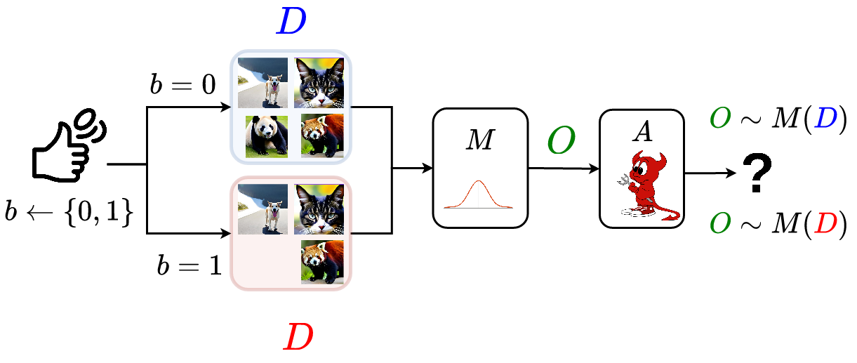
Differential Privacy as Hypothesis Testing
Hypothesis Testing is the defacto way of understanding how plausible is a given statement using the data that you have provided. The hypothesis that we want to prove is that an attacker is not effective against our $\epsilon$-DP algorithm and we can bound his performance using this guarantee. Consider the following binary hypothesis:
- $H_0$ (null) - $O \sim M(D_1)$
- $H_1$ (alternative) - $O \sim M(D_2)$
Define the error rates of the adversary:
- Type I Error (FNR) - $A$ calls that $D_1$ was used to compute $O$, but $D_2$ was used
- Type II Error (FPR) - $A$ calls that $D_2$ was used to compute $O$, but $D_1$ was used
Before going any further, please take a moment to take a look at the confusion matrix definition and how FNR and FPR are defined. I feel like this is one of the most confusing parts of statistics, don’t worry if you mix them up! A small reminder of the confusion matrix and its relationship with hypothesis testing:
| True Positive (TP) | False Positive (FP) | |
| True Negative (TN) | TPR = $\frac{TP}{TP + FN}$ | FNR = $\frac{FN}{TP + FN}$ |
| False Negative(FN) | FPR = $\frac{FP}{TN + FP}$ | TNR = $\frac{TN}{TN + FP}$ |
Returning to our problem, the question is: What does it mean for an adversary to be succesful? It should achieve both small FNR and FPR, meaning that it can properly distinguish if the data of a user has been used or not. The seminal works of Zhang et al., Kairouz et al. gave us a strong property on the attacker performance - If an algorithm is $\epsilon$-DP, then the error rates respect the following bound:
\[FNR + e^\epsilon * FPR > 1\] \[FPR + e^\epsilon * FNR > 1\]Epsilon lower bounds mapping for the possible value ranges of FPR and FNR in $\epsilon$-DP. This means that an attacker can have some regions, whom we will call trust regions, in which he is bounded to act, determined only by $\epsilon$.

Approximate DP
Approximate DP is a relaxation to the pure-DP formulation in which we use a negligible term $\delta$ to describe a catastrophic failure, for example, leaking a part of the private data. This type of relaxation is common in cryptography to achieve practicality, as $\epsilon$-DP is both restrictive and hard on utility. Keeping the notation and above $(\epsilon, \delta)$-DP is defined as:
\[P[M(D_1) \in O] < e^\epsilon * P[M(D_2) \in O] + \delta\]This makes the overall guarantees harder to understand. Let’s use look at it through the lens of privacy profiles:We can observe how this formulation makes our analysis of the performance of an attacker a bit more tedious, as we have a new parameter to take into account when trying to understand the trust region in which an attacker is allowed to perform. Let’s plot them for fixed values of $\delta$!
.png?raw=true)
Observe how the region between the blue dotted line and the 0 epsilon marker line evolves. When $\delta$=0, they overlap, we are in the same case as $\epsilon$-DP. As delta increases, there is a region between the $\epsilon=0$ line and the blue dotted line that is considered perfectly private. This gives relaxation to our epsilon needs (but we decide to ignore a part of the behaviour of the attacker. This is why epsilon has to be cryptographically small, it is a useful tool for tail bounding very improbable scenarios, but we don’t want to allow too many of them!
End Note
I think this is enough information for one sitting, we have a good basis for understanding how adversaries are bounded to performa against $\epsilon$-DP or $(\epsilon, \delta)$-DP mechanisms. The challenger doesn’t care about either the data or the attacker’s knowledge, our defence mechanism is a worst-case scenario one, good luck on breaking that! Using this primitive, one can understand new fundamental mechanisms:
- Trust regions are used to derive the optimal composition:
- Can we evaluate the epsilon that an algorithm provides against an instantiable adversary?
- Generalize $(\epsilon, \delta)$-DP using all the achievable privacy profiles for a mechanism a la f-DP
